A Beginner Random Random Forest Tutorial
When I have a data project in mind and have no idea on where to start modeling, I will always use the Random Forest model. It is not because of its catchy name
and the fact that I always misspell it as Rain Forest, it is quick, convenient, easy to understand and, it provides decent results. Isn't it cool? Yes, it is! So we are going to discuss more
RainRandom Forest details in this post.
What is Random Forest model?
First thing first, from the words of Random Forest, we know that this model is about a lot of trees (so is rain forest, that is why I keep linking rain forest as random forest...). And the "tree" in the Random Forest model is actually a decision tree. Let's pick our Titanic Survivors project as an example, a decision tree should look like:
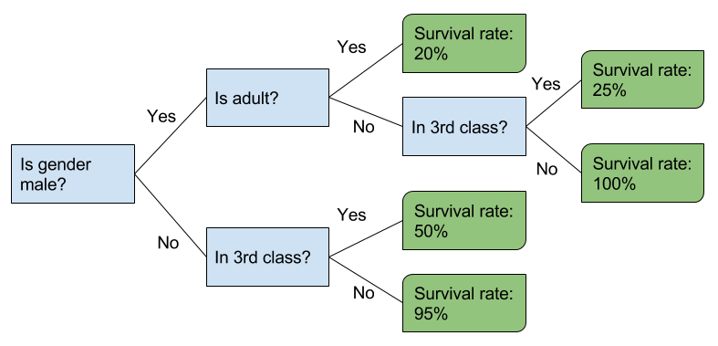
The advantage of using decision tree is its simplicity, we can observe the results graphically without having a statistics background. It is also very fast to build and test in development environment.
Now we have a tree, then what's next? We can't call a place "forest" with just one tree. So the Random Forest model is a model that consists of many decision trees. You may hear "all men are created equal", but in Random Forest,
All trees are created unequal
The decision trees in a Random Forest model are created randomly. The model splits a node among a random subset of features, then creates certain number of trees (depending on the model parameter, the default number of trees in sklearn Random Forest library is 10).

The rationales behind this setting are:
- making weak or uncorrelated sub-models for ensemble
- eliminating an overfitting issue on a tree model
Advantages of Random Forest
We have tried to use ensemble technique to get a better prediction on the Iowa House Prices project. The same thing happens in the Random Forest model, but this time, the model just does the ensemble itself. The RF model creates trees and calculates votes from each tree. Since those trees are less correlated, the RF model is able to reduce variance and find a better prediction through majority voting.
And a tree based model is considered as a greedy model. As it always aims to find the optimal solution for each smaller instance and reduce training data error. The tree model turns out splitting too many nodes and making the model too specified for certain features. Thus, it increases the testing data set error. The Random Forest model can eliminate overfitting issue because the model is not split by all features in the data set, but random subsets of those features. Every snowflake tree is unique in the Random Forest, the ensemble of variance is then smaller than the variance of an individual model.
Other than that, the Random Forest model can also compute feature importance for feature selection process. Let's use the Titanic project as an example:
import pandas as pd from sklearn.ensemble import RandomForestClassifier #load the train data set df_train = pd.read_csv("../input/train.csv") #prepare training data, remove unused fields train_x = df_train.drop(['Survived', 'PassengerId', 'Name', 'Ticket'], axis=1)train_x = df_train.drop(['Survived', 'PassengerId', 'Name', 'Ticket'], axis=1) train_y = df_train['Survived'] #convert all values to numeric values train_x_all_num = (train_x.apply(lambda x: pd.factorize(x)[0])) model = RandomForestClassifier() model.fit(train_x_all_num, train_y) #get feature importance from Random Forest importances = model.feature_importances_ print ("Sorted Feature Importance:") sorted_feature_importance = sorted(zip(importances, list(train_x_all_num)), reverse=True) print (sorted_feature_importance)
And get the following results:
Sorted Feature Importance: [(0.24543182417104634, 'Sex'), (0.22380032382910783, 'Age'), (0.20791521450928369, 'Fare'), (0.10294078976088994, 'Cabin'), (0.080212751900751736, 'Pclass'), (0.054506067168341811, 'Parch'), (0.045022270592417118, 'SibSp'), (0.040170758068161436, 'Embarked')]
Limitations of Random Forest
The Random Forest model is good because it comprises a fair model with randomly generated decision trees. However, its randomness also becomes its badness. We may input the number of trees, number of maximum features and the maximum depth of a tree for the RF model. But we just don't know how exactly it plants a tree and comes up with the prediction. We can only know the prediction is a majority of the generated decision trees.

Another limitation for the RF model is, extrapolation. Actually, it is not just a limitation for the RF model, but for all tree-based models. A linear regression model, like the tipping model we mentioned, can predict a trend for the tips. While a decision tree model can only predict the outcomes from data previously encountered. As the decision tree makes a decision based on the form of "if input > value then go left, otherwise go right", likes the following diagram:
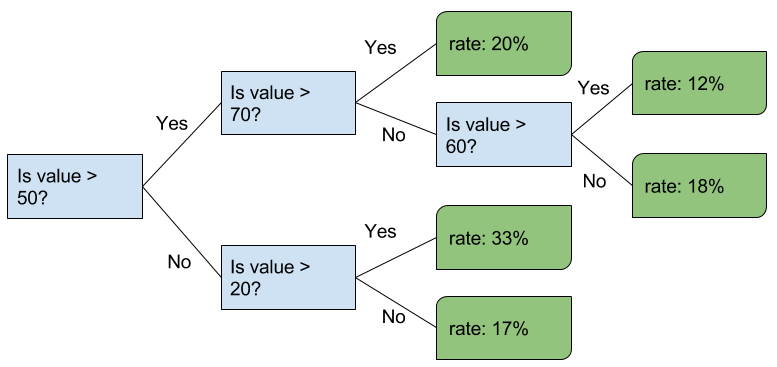
No matter an input is 71 or 70001, the result is always 20%. When the testing data is out of the range of the training data, it will be treated in the same manner as the minimal/maximal value already encountered in the training data set.
What have we learnt in this post?
- Introduction of the RF model
- Advantages of RF
- Limitation of RF
- Is it just me who always misspell Random Forest as Rain Forest??


